SAS exercise The data in RICEDATAxlsx was adapted from USDA

SAS exercise

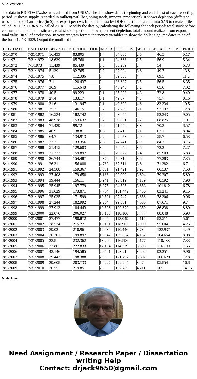
The data in RICEDATA.xlsx was adapted from USDA. The data show dates (beginning and end dates) of each reporting period. It shows supply, recorded in million(cwt) (beginning stock, imports, production). It shows depletion (different uses and export) and price (in $) for export per cwt. Import the data by DDE direct file transfer into SAS to create a file called RICE in LIBRARY called AGRIC. Modify the data by calculating the following for each period: total stock before consumption, total domestic use, total stock depletion, leftover, percent depletion, total amount realized from export, total value (in $) of production. In your program format the money variables to show the dollar sign, the dates to be of the form 12-13-1999. Output the modified file.

BEG_DATE	END_DATE	BEG_STOCK	PRODUCTION	IMPORT	FOOD_USE	SEED_USE	EXPORT_USE	PRICE
8/1/1970	7/31/1971	16.439	83.805	1.4	34.005	2.5	46.5	5.17
8/1/1971	7/31/1972	18.639	85.768	1.1	34.668	2.5	56.9	5.34
8/1/1972	7/1/1973	11.439	85.439	0.5	35.239	3	54	6.73
8/1/1973	7/31/1974	5.139	92.765	0.2	37.004	3.6	49.7	13.8
8/1/1974	7/31/1975	7.8	112.386	0	39.586	4	69.5	11.2
8/1/1975	7/31/1976	7.1	128.437	0	38.637	3.5	56.5	8.35
8/1/1976	7/31/1977	36.9	115.648	0	43.248	3.2	65.6	7.02
8/1/1977	7/31/1978	40.5	99.223	0.1	35.323	4.3	72.8	9.49
8/1/1978	7/31/1979	27.4	133.17	0.1	49.07	4.3	75.7	8.16
8/1/1979	7/31/1980	31.6	131.947	0.1	49.803	4.8	83.334	10.5
8/1/1980	7/31/1981	25.7	146.15	0.2	57.289	5.1	93.137	12.8
8/1/1981	7/31/1982	16.534	182.742	0.4	63.955	4.4	82.343	9.05
8/1/1982	7/31/1983	48.978	153.637	0.7	59.851	3.2	68.825	7.91
8/1/1983	7/31/1984	71.439	99.72	0.9	51.559	3.3	70.3	8.57
8/1/1984	7/31/1985	46.9	138.81	1.6	57.41	3.1	62.1	8.04
8/1/1985	7/31/1986	64.7	134.913	2.2	62.873	2.94	58.7	6.53
8/1/1986	7/31/1987	77.3	133.356	2.6	74.741	2.9	84.2	3.75
8/1/1987	7/31/1988	51.415	129.603	3	76.846	3.6	72.2	7.27
8/1/1988	7/31/1989	31.372	159.897	3.8	79.022	3.4	85.903	6.83
8/1/1989	7/31/1990	26.744	154.487	4.378	78.316	3.6	77.383	7.35
8/1/1990	7/31/1991	26.31	156.088	4.783	87.611	3.6	71.382	6.7
8/1/1991	7/31/1992	24.588	159.367	5.331	91.421	3.92	66.537	7.58
8/1/1992	7/31/1993	27.408	179.658	6.188	90.999	3.604	79.207	5.89
8/1/1993	7/31/1994	39.444	156.11	6.941	93.819	4.139	78.592	7.98
8/1/1994	7/31/1995	25.945	197.779	8.075	94.505	3.853	101.812	6.78
8/1/1995	7/31/1996	31.629	173.871	7.704	101.442	3.486	83.241	9.15
8/1/1996	7/31/1997	25.035	171.599	10.521	97.747	3.858	78.306	9.96
8/1/1997	7/31/1998	27.244	182.992	9.264	99.861	4.055	87.671	9.7
8/1/1998	7/31/1999	27.913	184.443	10.596	109.679	4.359	86.838	8.89
8/1/1999	7/31/2000	22.076	206.027	10.105	118.106	3.777	88.848	5.93
8/1/2000	7/31/2001	27.477	190.872	10.85	113.049	4.115	83.511	5.61
8/1/2001	7/31/2002	28.524	215.27	13.191	118.962	3.999	95.004	4.25
8/1/2002	7/31/2003	39.02	210.96	14.834	110.446	3.73	123.937	4.49
8/1/2003	7/31/2004	26.701	199.897	15.042	109.054	4.132	104.654	8.08
8/1/2004	7/31/2005	23.8	232.362	13.204	116.896	4.177	110.433	7.33
8/1/2005	7/31/2006	37.86	222.833	17.134	114.379	3.503	116.799	7.65
8/1/2006	7/31/2007	43.146	194.585	20.581	123.21	3.408	92.251	9.96
8/1/2007	7/31/2008	39.443	198.388	23.9	121.797	3.697	106.629	12.8
8/1/2008	7/31/2009	29.608	203.733	19.227	122.294	3.87	95.854	16.8
8/1/2009	7/31/2010	30.55	219.85	20	132.789	4.211	105	14.15

Solution

a generation chief is in charge of booking the month to month creation levels

of a specific item for an arranging skyline of twelve months. For arranging purposes, the

administrator was given the accompanying data:

• The aggregate interest for the item in month j is dj , for j = 1, 2, . . ., 12. These could

either be focused on qualities or be founded on figures.

• The cost of creating every unit of the item in month j is cj (dollars), for j = 1,

2, . . ., 12. There is no setup/altered cost for generation.

• The stock holding cost per unit for month j is hj (dollars), for j = 1, 2, . . ., 12.

These are caused toward the end of every month.

• The creation limit for month j is mj , for j = 1, 2, . . ., 12.

The chief\'s undertaking is to create a generation calendar that minimizes the aggregate generation

furthermore, stock holding costs over this twelve-month arranging skyline.

To encourage the detailing of a direct program, the administrator chooses to make the accompanying

improving suppositions:

1. There is no underlying stock toward the start of the main month.

2. Units planned for creation in month j are quickly accessible for conveyance at

the start of that month. This implies as a result that the creation rate is vast.

3. Deficiency of the item is not permitted toward the end of any month.

To comprehend things better, let us consider the main month. Assume, for that month, the

arranged generation level equivalents 100 units and the request, d1, parallels 60 units. At that point, since

the underlying stock is 0 (Assumption 1), the closure stock level for the primary month

would be 0 + 100 60 = 40 units. Take note of that every one of the 100 units are quickly accessible for

conveyance (Assumption 2); and that given d1 = 60, one must deliver no under 60 units

in the main month, to dodge lack (Assumption 3). Assume facilitate that c1 = 15 and

h1 = 3. At that point, the aggregate cost for the primary month can be processed as: 15×100+3×40 = 1380

dollars.

Toward the begin of the second month, there would be 40 units of the item in stock,

what\'s more, the relating finishing stock can be processed comparably, in light of the underlying

stock, the planned creation level, and the aggregate interest for that month. The same

plan is then rehashed until the end of the whole arranging skyline.

1

We now continue with a direct programming (LP) plan of this issue.

The Decision Variables

The chief\'s assignment is to set a creation level for every month. Accordingly, we have twelve

choice factors:

xj = the creation level for month j, j = 1, 2, . . ., 12.

The Objective Function

Consider the main month once more. From the examination above, we have:

The generation cost measures up to c1x1.

The stock holding cost measures up to h1(x1 d1), accepting that the closure stock level,

x1 d1, is nonnegative.

Subsequently, the aggregate cost for the principal month breaks even with c1x1 + h1(x1 d1).

For the second month, we have:

The generation cost levels with c2x2.

The stock holding cost measures up to h2(x1d1+x2d2), expecting that the consummation stock

level, x1 d1 + x2 d2, is nonnegative. This takes after from the way that the beginning

stock level during the current month is x1 d1, the generation level during the current month is x2,

what\'s more, the interest during the current month is d2.

Consequently, the aggregate cost for the second month measures up to c2x2 + h2(x1 d1 + x2 d2).

Continuation of this contention yields that:

The aggregate creation cost for the whole arranging skyline measures up to

X

12

j=1

cjxj c1x1 + c2x2 + . . . + c12x12 ,

where we have presented the standard summation documentation (\"\" implies by definition).