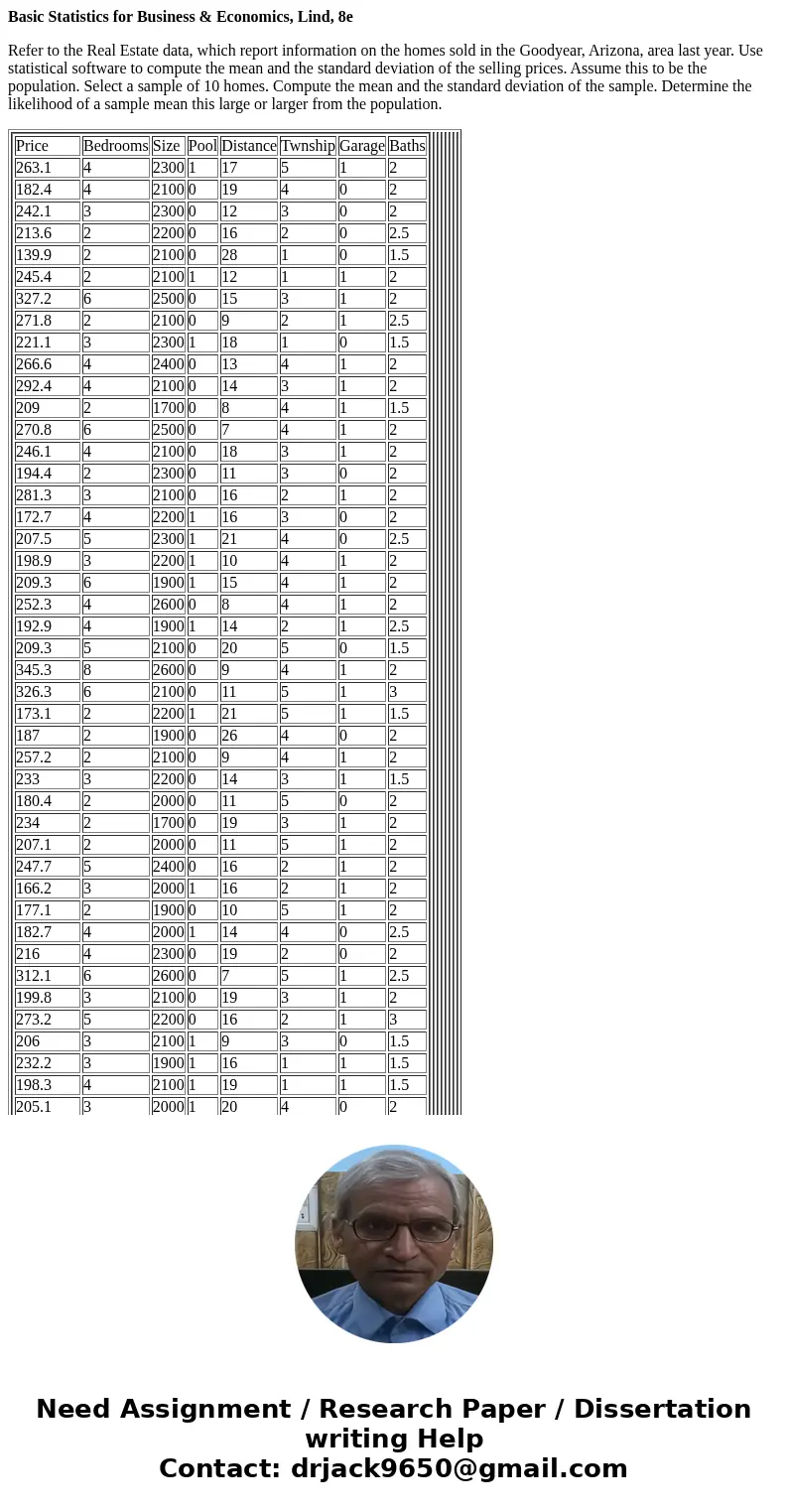
Basic Statistics for Business Economics Lind 8e Refer to th

Basic Statistics for Business & Economics, Lind, 8e

Refer to the Real Estate data, which report information on the homes sold in the Goodyear, Arizona, area last year. Use statistical software to compute the mean and the standard deviation of the selling prices. Assume this to be the population. Select a sample of 10 homes. Compute the mean and the standard deviation of the sample. Determine the likelihood of a sample mean this large or larger from the population.

Solution

The code for computation in R - statistical software are as follows.

Note:- The data given above was saved in the file named RealEstate.Goodyear.csv

The link for csv file is https://www.dropbox.com/s/3xi8w9swpqayw9l/RealEstate.Goodyear.csv?dl=0

> data<-read.csv(\"RealEstate.Goodyear.csv\")

This reads the data and saves it into a variable data frame named data.

> price<-data$Price

> mean(price)
[1] 221.1029
> sd(price)
[1] 47.1054

Thus the mean is 221.1029 and the standard deviation is 47.1054.

Now for the next step we have to select 10 random samples from the given data and compute their mean and standard deviation.

> t<-sample(price,10)
> t
[1] 269.9 327.2 173.6 176.0 252.3 240.0 227.1 271.8 172.4 245.4
> mean(t)
[1] 235.57
> sd(t)
[1] 50.25979

Here we can see that the mean obtained is larger than the mean calculated for the whole population.

Now the next part of the question asks the probability of mean of this random sample of 10 (which in this particular case is computed to be 235.57 ) being greater than the mean of population (which is 221.1029).

To do this we will create random samples of size 10 calculate their mean and if the mean is greater than 221.1029 then count it as 1. Repeat this process for 1000 times and, then the required probability will be given by count/1000.

> count<-0
> for (n in 1:1000){ if(mean(sample(prc,10))>221.1029){count=count+1}}
> count
[1] 493

Thus the required probability is 493/1000 = 0.493.

Download the csv file and you can repeat these steps yourself to get a better understanding.