For a random sample of dierent car models the average gas mi

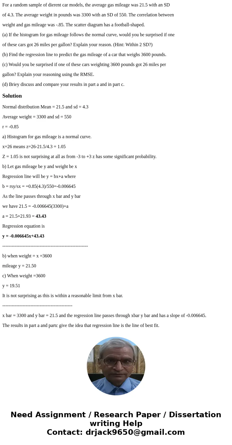
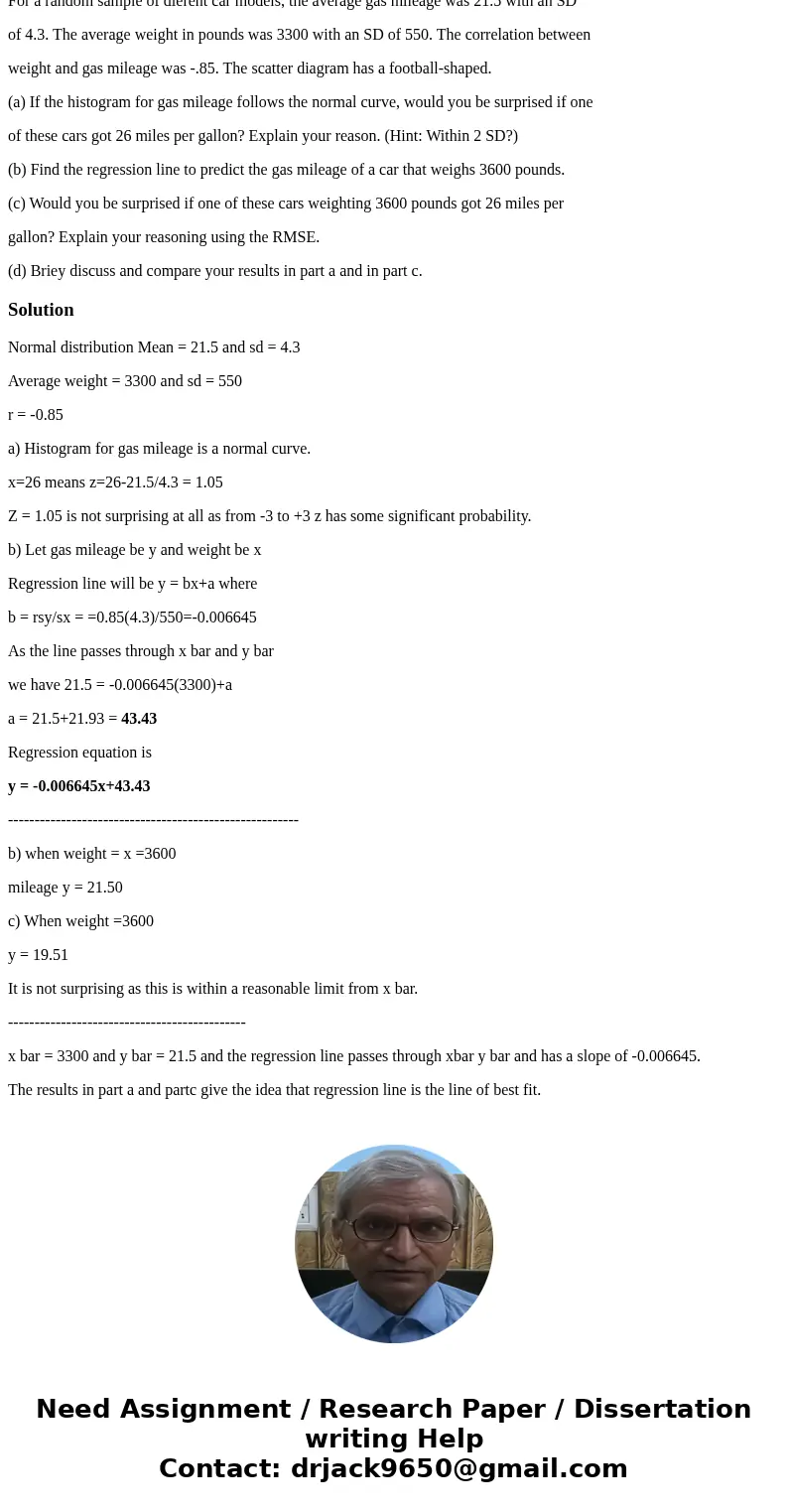
For a random sample of dierent car models, the average gas mileage was 21.5 with an SD

of 4.3. The average weight in pounds was 3300 with an SD of 550. The correlation between

weight and gas mileage was -.85. The scatter diagram has a football-shaped.

(a) If the histogram for gas mileage follows the normal curve, would you be surprised if one

of these cars got 26 miles per gallon? Explain your reason. (Hint: Within 2 SD?)

(b) Find the regression line to predict the gas mileage of a car that weighs 3600 pounds.

gallon? Explain your reasoning using the RMSE.

(d) Briey discuss and compare your results in part a and in part c.

Normal distribution Mean = 21.5 and sd = 4.3

Average weight = 3300 and sd = 550

r = -0.85

a) Histogram for gas mileage is a normal curve.

x=26 means z=26-21.5/4.3 = 1.05

Z = 1.05 is not surprising at all as from -3 to +3 z has some significant probability.

b) Let gas mileage be y and weight be x

Regression line will be y = bx+a where

b = rsy/sx = =0.85(4.3)/550=-0.006645

As the line passes through x bar and y bar

we have 21.5 = -0.006645(3300)+a

a = 21.5+21.93 = 43.43

Regression equation is

y = -0.006645x+43.43

-------------------------------------------------------

b) when weight = x =3600

mileage y = 21.50

c) When weight =3600

y = 19.51

It is not surprising as this is within a reasonable limit from x bar.

---------------------------------------------

x bar = 3300 and y bar = 21.5 and the regression line passes through xbar y bar and has a slope of -0.006645.

The results in part a and partc give the idea that regression line is the line of best fit.