Question 3 Perform a regression analysis using compa as the
Question 3)
Perform a regression analysis using compa as the dependent variable and the same independent variables as used in question 2. Show the result, and interpret your findings by answering the same questions.
Note: be sure to include the appropriate hypothesis statements.
A ) Regression hypotheses
Ho:
Ha:
Coefficient hyhpotheses (one to stand for all the separate variables)
Ho:
Ha:
B )Interpretation:
For the Regression as a whole:
What is the value of the F statistic:
What is the p-value associated with this value:
Is the p-value < 0.05?
Do you reject or not reject the null hypothesis:
What does this decision mean for our equal pay question (Do M and F get paid equaly?):
C )For each of the coefficients: Intercept, Midpoint, Age, Perf. rating, Service, Gender, Degree
What is the coefficient\'s p-value for each of the variables:
Is the p-value < 0.05?
Do you reject or not reject each null hypothesis:
What are the coefficients for the significant variables?
Using only the significant variables, what is the equation? Compa =
Is gender a significant factor in compa:
If so, who gets paid more with all other things being equal?
How do we know?
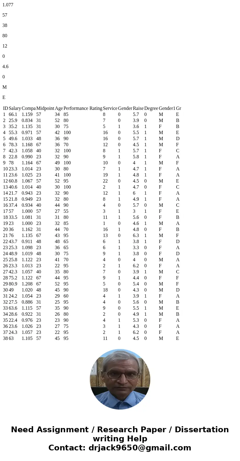
ID
Salary
Compa
Midpoint
Age
Performance Rating
Service
Gender
Raise
Degree
Gender1
Gr
1
66.1
1.159
57
34
85
8
0
5.7
0
M
E
2
25.9
0.834
31
52
80
7
0
3.9
0
M
B
3
35.2
1.135
31
30
75
5
1
3.6
1
F
B
4
55.3
0.971
57
42
100
16
0
5.5
1
M
E
5
49.6
1.033
48
36
90
16
0
5.7
1
M
D
6
78.3
1.168
67
36
70
12
0
4.5
1
M
F
7
42.3
1.058
40
32
100
8
1
5.7
1
F
C
8
22.8
0.990
23
32
90
9
1
5.8
1
F
A
9
78
1.164
67
49
100
10
0
4
1
M
F
10
23.3
1.014
23
30
80
7
1
4.7
1
F
A
11
23.6
1.025
23
41
100
19
1
4.8
1
F
A
12
60.8
1.067
57
52
95
22
0
4.5
0
M
E
13
40.6
1.014
40
30
100
2
1
4.7
0
F
C
14
21.7
0.943
23
32
90
12
1
6
1
F
A
15
21.8
0.949
23
32
80
8
1
4.9
1
F
A
16
37.4
0.934
40
44
90
4
0
5.7
0
M
C
17
57
1.000
57
27
55
3
1
3
1
F
E
18
33.5
1.081
31
31
80
11
1
5.6
0
F
B
19
23
1.000
23
32
85
1
0
4.6
1
M
A
20
36
1.162
31
44
70
16
1
4.8
0
F
B
21
76
1.135
67
43
95
13
0
6.3
1
M
F
22
43.7
0.911
48
48
65
6
1
3.8
1
F
D
23
25.3
1.098
23
36
65
6
1
3.3
0
F
A
24
48.9
1.019
48
30
75
9
1
3.8
0
F
D
25
25.8
1.122
23
41
70
4
0
4
0
M
A
26
23.3
1.013
23
22
95
2
1
6.2
0
F
A
27
42.3
1.057
40
35
80
7
0
3.9
1
M
C
28
75.2
1.122
67
44
95
9
1
4.4
0
F
F
29
80.9
1.208
67
52
95
5
0
5.4
0
M
F
30
49
1.020
48
45
90
18
0
4.3
0
M
D
31
24.2
1.054
23
29
60
4
1
3.9
1
F
A
32
27.5
0.886
31
25
95
4
0
5.6
0
M
B
33
63.6
1.115
57
35
90
9
0
5.5
1
M
E
34
28.6
0.922
31
26
80
2
0
4.9
1
M
B
35
22.4
0.976
23
23
90
4
1
5.3
0
F
A
36
23.6
1.026
23
27
75
3
1
4.3
0
F
A
37
24.3
1.057
23
22
95
2
1
6.2
0
F
A
38
63
1.105
57
45
95
11
0
4.5
0
M
E
39
34.8
1.123
31
27
90
6
1
5.5
0
F
B
40
24.3
1.057
23
24
90
2
0
6.3
0
M
A
41
42.8
1.071
40
25
80
5
0
4.3
0
M
C
42
23
0.998
23
32
100
8
1
5.7
1
F
A
43
75.4
1.125
67
42
95
20
1
5.5
0
F
F
44
60.7
1.065
57
45
90
16
0
5.2
1
M
E
45
57.9
1.206
48
36
95
8
1
5.2
1
F
D
46
62.2
1.091
57
39
75
20
0
3.9
1
M
E
47
62.2
1.091
57
37
95
5
0
5.5
1
M
E
48
70.1
1.230
57
34
90
11
1
5.3
1
F
E
49
61.7
1.083
57
41
95
21
0
6.6
0
M
E
50
61.4
1.077
57
38
80
12
0
4.6
0
M
E
| ID | Salary | Compa | Midpoint | Age | Performance Rating | Service | Gender | Raise | Degree | Gender1 | Gr |
| 1 | 66.1 | 1.159 | 57 | 34 | 85 | 8 | 0 | 5.7 | 0 | M | E |
| 2 | 25.9 | 0.834 | 31 | 52 | 80 | 7 | 0 | 3.9 | 0 | M | B |
| 3 | 35.2 | 1.135 | 31 | 30 | 75 | 5 | 1 | 3.6 | 1 | F | B |
| 4 | 55.3 | 0.971 | 57 | 42 | 100 | 16 | 0 | 5.5 | 1 | M | E |
| 5 | 49.6 | 1.033 | 48 | 36 | 90 | 16 | 0 | 5.7 | 1 | M | D |
| 6 | 78.3 | 1.168 | 67 | 36 | 70 | 12 | 0 | 4.5 | 1 | M | F |
| 7 | 42.3 | 1.058 | 40 | 32 | 100 | 8 | 1 | 5.7 | 1 | F | C |
| 8 | 22.8 | 0.990 | 23 | 32 | 90 | 9 | 1 | 5.8 | 1 | F | A |
| 9 | 78 | 1.164 | 67 | 49 | 100 | 10 | 0 | 4 | 1 | M | F |
| 10 | 23.3 | 1.014 | 23 | 30 | 80 | 7 | 1 | 4.7 | 1 | F | A |
| 11 | 23.6 | 1.025 | 23 | 41 | 100 | 19 | 1 | 4.8 | 1 | F | A |
| 12 | 60.8 | 1.067 | 57 | 52 | 95 | 22 | 0 | 4.5 | 0 | M | E |
| 13 | 40.6 | 1.014 | 40 | 30 | 100 | 2 | 1 | 4.7 | 0 | F | C |
| 14 | 21.7 | 0.943 | 23 | 32 | 90 | 12 | 1 | 6 | 1 | F | A |
| 15 | 21.8 | 0.949 | 23 | 32 | 80 | 8 | 1 | 4.9 | 1 | F | A |
| 16 | 37.4 | 0.934 | 40 | 44 | 90 | 4 | 0 | 5.7 | 0 | M | C |
| 17 | 57 | 1.000 | 57 | 27 | 55 | 3 | 1 | 3 | 1 | F | E |
| 18 | 33.5 | 1.081 | 31 | 31 | 80 | 11 | 1 | 5.6 | 0 | F | B |
| 19 | 23 | 1.000 | 23 | 32 | 85 | 1 | 0 | 4.6 | 1 | M | A |
| 20 | 36 | 1.162 | 31 | 44 | 70 | 16 | 1 | 4.8 | 0 | F | B |
| 21 | 76 | 1.135 | 67 | 43 | 95 | 13 | 0 | 6.3 | 1 | M | F |
| 22 | 43.7 | 0.911 | 48 | 48 | 65 | 6 | 1 | 3.8 | 1 | F | D |
| 23 | 25.3 | 1.098 | 23 | 36 | 65 | 6 | 1 | 3.3 | 0 | F | A |
| 24 | 48.9 | 1.019 | 48 | 30 | 75 | 9 | 1 | 3.8 | 0 | F | D |
| 25 | 25.8 | 1.122 | 23 | 41 | 70 | 4 | 0 | 4 | 0 | M | A |
| 26 | 23.3 | 1.013 | 23 | 22 | 95 | 2 | 1 | 6.2 | 0 | F | A |
| 27 | 42.3 | 1.057 | 40 | 35 | 80 | 7 | 0 | 3.9 | 1 | M | C |
| 28 | 75.2 | 1.122 | 67 | 44 | 95 | 9 | 1 | 4.4 | 0 | F | F |
| 29 | 80.9 | 1.208 | 67 | 52 | 95 | 5 | 0 | 5.4 | 0 | M | F |
| 30 | 49 | 1.020 | 48 | 45 | 90 | 18 | 0 | 4.3 | 0 | M | D |
| 31 | 24.2 | 1.054 | 23 | 29 | 60 | 4 | 1 | 3.9 | 1 | F | A |
| 32 | 27.5 | 0.886 | 31 | 25 | 95 | 4 | 0 | 5.6 | 0 | M | B |
| 33 | 63.6 | 1.115 | 57 | 35 | 90 | 9 | 0 | 5.5 | 1 | M | E |
| 34 | 28.6 | 0.922 | 31 | 26 | 80 | 2 | 0 | 4.9 | 1 | M | B |
| 35 | 22.4 | 0.976 | 23 | 23 | 90 | 4 | 1 | 5.3 | 0 | F | A |
| 36 | 23.6 | 1.026 | 23 | 27 | 75 | 3 | 1 | 4.3 | 0 | F | A |
| 37 | 24.3 | 1.057 | 23 | 22 | 95 | 2 | 1 | 6.2 | 0 | F | A |
| 38 | 63 | 1.105 | 57 | 45 | 95 | 11 | 0 | 4.5 | 0 | M | E |
| 39 | 34.8 | 1.123 | 31 | 27 | 90 | 6 | 1 | 5.5 | 0 | F | B |
| 40 | 24.3 | 1.057 | 23 | 24 | 90 | 2 | 0 | 6.3 | 0 | M | A |
| 41 | 42.8 | 1.071 | 40 | 25 | 80 | 5 | 0 | 4.3 | 0 | M | C |
| 42 | 23 | 0.998 | 23 | 32 | 100 | 8 | 1 | 5.7 | 1 | F | A |
| 43 | 75.4 | 1.125 | 67 | 42 | 95 | 20 | 1 | 5.5 | 0 | F | F |
| 44 | 60.7 | 1.065 | 57 | 45 | 90 | 16 | 0 | 5.2 | 1 | M | E |
| 45 | 57.9 | 1.206 | 48 | 36 | 95 | 8 | 1 | 5.2 | 1 | F | D |
| 46 | 62.2 | 1.091 | 57 | 39 | 75 | 20 | 0 | 3.9 | 1 | M | E |
| 47 | 62.2 | 1.091 | 57 | 37 | 95 | 5 | 0 | 5.5 | 1 | M | E |
| 48 | 70.1 | 1.230 | 57 | 34 | 90 | 11 | 1 | 5.3 | 1 | F | E |
| 49 | 61.7 | 1.083 | 57 | 41 | 95 | 21 | 0 | 6.6 | 0 | M | E |
| 50 | 61.4 | 1.077 | 57 | 38 | 80 | 12 | 0 | 4.6 | 0 | M | E |
Solution
Here regression hypothesis is,
H0 : 1 = 2 = · · · = p = 0 Vs H1 : j 0
for at least for at least one j , j = 1,2,......p
Here we use F-statistics.
Coefficient hypothesis :
H0 : j = 0 Vs H1 : j 0
Here we use t-statistics.
All the given questions we are done using MINITAB.
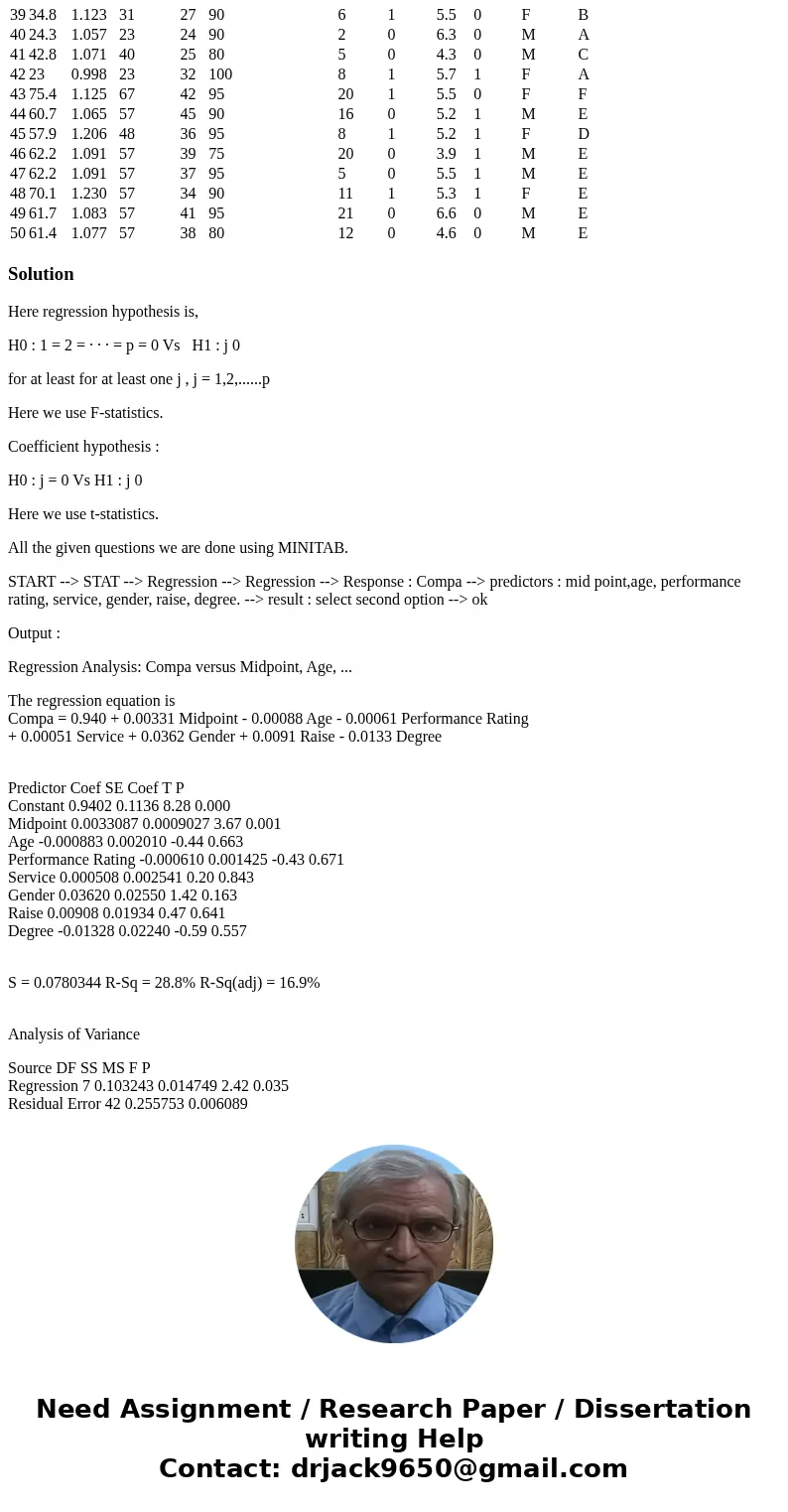
START --> STAT --> Regression --> Regression --> Response : Compa --> predictors : mid point,age, performance rating, service, gender, raise, degree. --> result : select second option --> ok
Output :
Regression Analysis: Compa versus Midpoint, Age, ...
The regression equation is
Compa = 0.940 + 0.00331 Midpoint - 0.00088 Age - 0.00061 Performance Rating
+ 0.00051 Service + 0.0362 Gender + 0.0091 Raise - 0.0133 Degree
Predictor Coef SE Coef T P
Constant 0.9402 0.1136 8.28 0.000
Midpoint 0.0033087 0.0009027 3.67 0.001
Age -0.000883 0.002010 -0.44 0.663
Performance Rating -0.000610 0.001425 -0.43 0.671
Service 0.000508 0.002541 0.20 0.843
Gender 0.03620 0.02550 1.42 0.163
Raise 0.00908 0.01934 0.47 0.641
Degree -0.01328 0.02240 -0.59 0.557
S = 0.0780344 R-Sq = 28.8% R-Sq(adj) = 16.9%
Analysis of Variance
Source DF SS MS F P
Regression 7 0.103243 0.014749 2.42 0.035
Residual Error 42 0.255753 0.006089
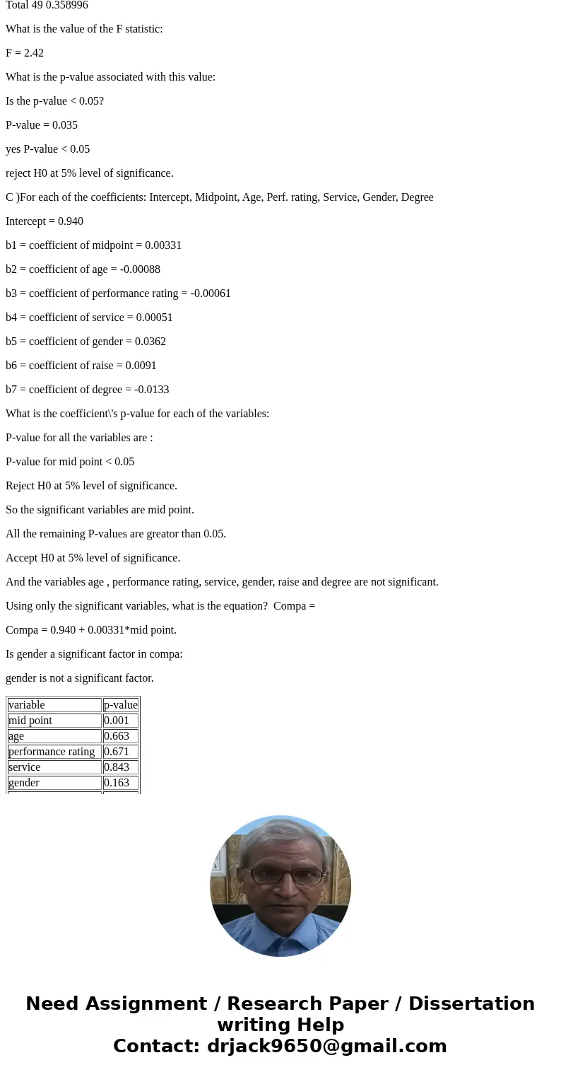
Total 49 0.358996
What is the value of the F statistic:
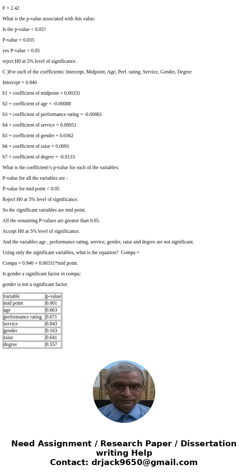
F = 2.42
What is the p-value associated with this value:
Is the p-value < 0.05?
P-value = 0.035
yes P-value < 0.05
reject H0 at 5% level of significance.
C )For each of the coefficients: Intercept, Midpoint, Age, Perf. rating, Service, Gender, Degree
Intercept = 0.940
b1 = coefficient of midpoint = 0.00331
b2 = coefficient of age = -0.00088
b3 = coefficient of performance rating = -0.00061
b4 = coefficient of service = 0.00051
b5 = coefficient of gender = 0.0362
b6 = coefficient of raise = 0.0091
b7 = coefficient of degree = -0.0133
What is the coefficient\'s p-value for each of the variables:
P-value for all the variables are :
P-value for mid point < 0.05
Reject H0 at 5% level of significance.
So the significant variables are mid point.
All the remaining P-values are greator than 0.05.
Accept H0 at 5% level of significance.
And the variables age , performance rating, service, gender, raise and degree are not significant.
Using only the significant variables, what is the equation? Compa =
Compa = 0.940 + 0.00331*mid point.
Is gender a significant factor in compa:
gender is not a significant factor.
| variable | p-value |
| mid point | 0.001 |
| age | 0.663 |
| performance rating | 0.671 |
| service | 0.843 |
| gender | 0.163 |
| raise | 0.641 |
| degree | 0.557 |






 Homework Sourse