In the Week 4 assignment you were asked to build a multiple

In the Week 4 assignment, you were asked to build a multiple regression model to explain the variability in the median school year, using a minimum of seven independent variables. Using the same model, thoroughly assess your model\'s diagnostics. Identify all relevant assessment dimensions, briefly outline their purpose and importance, and provide an assessment of your model in terms of the identified diagnostic measures.

Week 4 submission

Correlation

Correlation

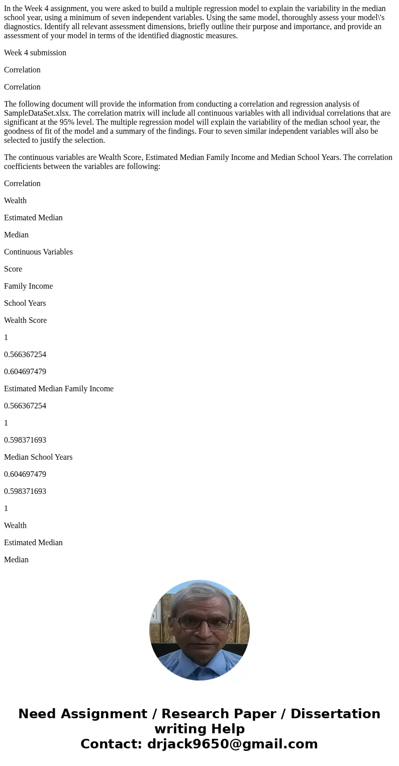
The following document will provide the information from conducting a correlation and regression analysis of SampleDataSet.xlsx. The correlation matrix will include all continuous variables with all individual correlations that are significant at the 95% level. The multiple regression model will explain the variability of the median school year, the goodness of fit of the model and a summary of the findings. Four to seven similar independent variables will also be selected to justify the selection.

The continuous variables are Wealth Score, Estimated Median Family Income and Median School Years. The correlation coefficients between the variables are following:

Correlation

Wealth  

Estimated Median

Median  

Continuous Variables

Score

Family Income

School Years

Wealth Score

1

0.566367254

0.604697479

Estimated Median Family Income

0.566367254

1

0.598371693

Median School Years

0.604697479

0.598371693

1

Wealth  

Estimated Median

Median  

Continuous Variables

Score

Family Income

School Years

Wealth Score

In

15.21207094

16.80640485

Estimated Median Family Income

15.21207094

Inf

16.5317197

Median School Years

16.80640485

16.5317197

Inf

Wealth  

Estimated Median

Median  

Continuous Variables

Score

Family Income

School Years

Wealth Score

0

2.21045

1.10055

Estimated Median Family Income

2.21045

0

2.06568

Median School Years

1.10055

2.06568

0

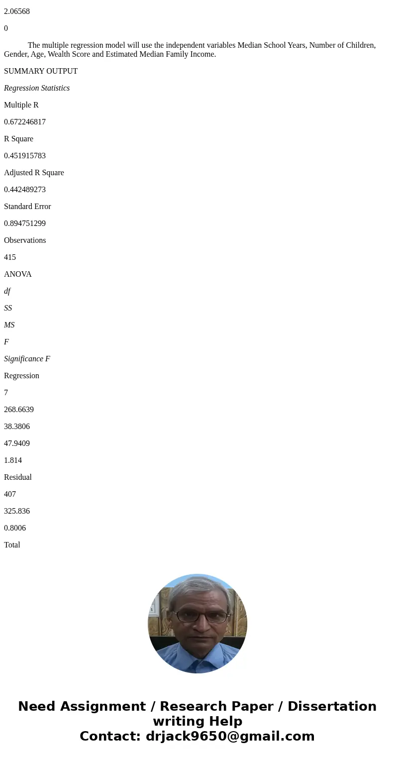
            The multiple regression model will use the independent variables Median School Years, Number of Children, Gender, Age, Wealth Score and Estimated Median Family Income.

SUMMARY OUTPUT

Regression Statistics

Multiple R

0.672246817

R Square

0.451915783

Adjusted R Square

0.442489273

Standard Error

0.894751299

Observations

415

ANOVA

df

SS

MS

F

Significance F

Regression

7

268.6639

38.3806

47.9409

1.814

Residual

407

325.836

0.8006

Total

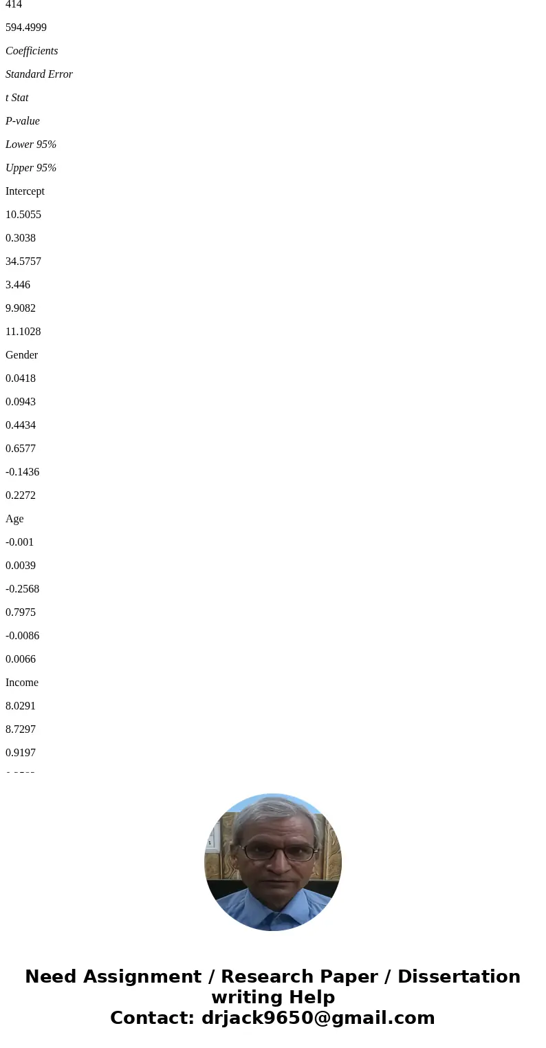
414

594.4999

Coefficients

Standard Error

t Stat

P-value

Lower 95%

Upper 95%

Intercept

10.5055

0.3038

34.5757

3.446

9.9082

11.1028

Gender

0.0418

0.0943

0.4434

0.6577

-0.1436

0.2272

Age

-0.001

0.0039

-0.2568

0.7975

-0.0086

0.0066

Income

8.0291

8.7297

0.9197

0.3582

-9.1318

2.519

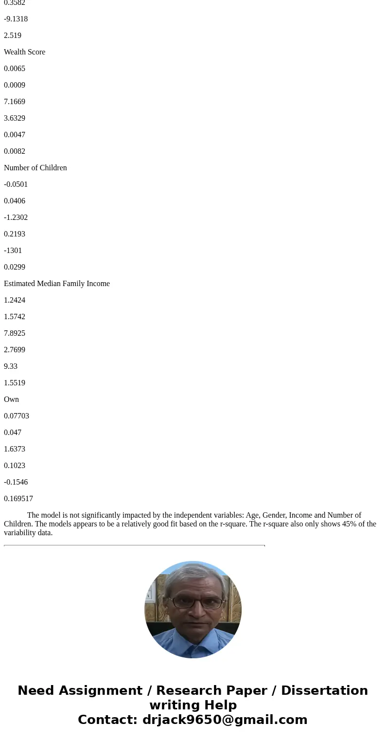
Wealth Score

0.0065

0.0009

7.1669

3.6329

0.0047

0.0082

Number of Children

-0.0501

0.0406

-1.2302

0.2193

-1301

0.0299

Estimated Median Family Income

1.2424

1.5742

7.8925

2.7699

9.33

1.5519

Own

0.07703

0.047

1.6373

0.1023

-0.1546

0.169517

            The model is not significantly impacted by the independent variables: Age, Gender, Income and Number of Children. The models appears to be a relatively good fit based on the r-square. The r-square also only shows 45% of the variability data.

Correlation
	Wealth	Estimated Median	Median
Continuous Variables	Score	Family Income	School Years
Wealth Score	1	0.566367254	0.604697479
Estimated Median Family Income	0.566367254	1	0.598371693
Median School Years	0.604697479	0.598371693	1
	Wealth	Estimated Median	Median
Continuous Variables	Score	Family Income	School Years
Wealth Score	In	15.21207094	16.80640485
Estimated Median Family Income	15.21207094	Inf	16.5317197
Median School Years	16.80640485	16.5317197	Inf

Solution

Our assesment based on the results are as follows

1) first of all we judge the goodness of fit using adjusted R-squared which is here only 44.24% approximately. This indicates that model fitting is not as good as expected. Only 44.24% (approx) of the total variation is explained or accounted for by the model used.

2) The model is not significantly impacted by the independent variables (viz. Age,Gender, No.of children, Income,wealth score,Estimated median family income etc,) since all the p-values corresponding to the variables are higher than .05 or .01. (usual level of significance).

3) However it was significant to perform regression.