2 Suppose we decide to include another independent variable
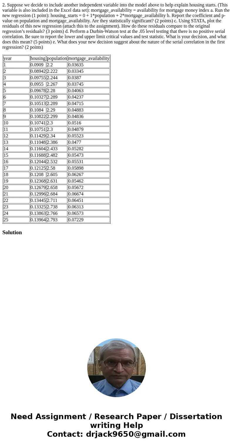
2. Suppose we decide to include another independent variable into the model above to help explain housing starts. (This variable is also included in the Excel data set): mortgage_availability = availability for mortgage money index a. Run the new regression (1 point): housing_starts = 0 + 1*population + 2*mortgage_availability b. Report the coefficient and p-value on population and mortgage_availability. Are they statistically significant? (2 points) c. Using STATA, plot the residuals of this new regression (attach this to the assignment). How do these residuals compare to the original regression’s residuals? (3 points) d. Perform a Durbin-Watson test at the .05 level testing that there is no positive serial correlation. Be sure to report the lower and upper limit critical values and test statistic. What is your decision, and what does this mean? (5 points) e. What does your new decision suggest about the nature of the serial correlation in the first regression? (2 points)
| year | housing | population | mortgage_availability |
| 1 | 0.0909 | 2.2 | 0.03635 |
| 2 | 0.08942 | 2.222 | 0.03345 |
| 3 | 0.09755 | 2.244 | 0.0387 |
| 4 | 0.0955 | 2.267 | 0.03745 |
| 5 | 0.09678 | 2.28 | 0.04063 |
| 6 | 0.10327 | 2.289 | 0.04237 |
| 7 | 0.10513 | 2.289 | 0.04715 |
| 8 | 0.1084 | 2.29 | 0.04883 |
| 9 | 0.10822 | 2.299 | 0.04836 |
| 10 | 0.10741 | 2.3 | 0.0516 |
| 11 | 0.10751 | 2.3 | 0.04879 |
| 12 | 0.11429 | 2.34 | 0.05523 |
| 13 | 0.11048 | 2.386 | 0.0477 |
| 14 | 0.11604 | 2.433 | 0.05282 |
| 15 | 0.11688 | 2.482 | 0.05473 |
| 16 | 0.12044 | 2.532 | 0.05531 |
| 17 | 0.12125 | 2.58 | 0.05898 |
| 18 | 0.1208 | 2.605 | 0.06267 |
| 19 | 0.12368 | 2.631 | 0.05462 |
| 20 | 0.12679 | 2.658 | 0.05672 |
| 21 | 0.12996 | 2.684 | 0.06674 |
| 22 | 0.13445 | 2.711 | 0.06451 |
| 23 | 0.13325 | 2.738 | 0.06313 |
| 24 | 0.13863 | 2.766 | 0.06573 |
| 25 | 0.13964 | 2.793 | 0.07229 |
Solution

 Homework Sourse