When one company buys another company it is not unusual that

When one company buys another company, it is not unusual that some workers are terminated. The severance benefits offered to the laid-off workers are often the subject of dispute. Suppose that the Laurier Company recently bought the Western Company and subsequently terminated 20 of Western’s employees. As part of the buyout agreement, it was promised that the severance packages offered to former Western employees would be equivalent to those offered to Laurier employees who had been terminated in the past year. Thirty-six-year-old Bill Smith, a Western employee for the past 10 years, earning $32,000 per year, was one of those let go. His severance package included an offer of 5 weeks’ severance pay. Bill complained that this offer was less than that offered to Laurier employees when they were laid off, in contravention of the buyout agreement. A statistician is called in to settle the dispute. The statistician is told that severance is determined by three factors: age, length of service with the company, and pay. To determine how generous the severance package had been, a random sample of 50 Laurier ex-employees was taken. For each, the following variables were recorded:

Number of weeks of severance pay (Weeks SP)

Age of employee (Age)

Number of years with the company (Years)

Annual pay (Pay)

Estimate the appropriate regression equation for Weeks SP with the data provided in the sheet entitled “Severance”.

Perform an analysis to determine whether Bill is correct in his assessment of the severance package (hint: Based on your regression estimates, how many weeks of severance pay would have been received by a Laurier worker with the same characteristics as Bill if Western employees had actually received the same types of severance packages as Laurier employees?)

Weeks SP	Weeks SP	Weeks SP	Weeks SP
13	13	13	13
13	13	13	13
11	11	11	11
14	14	14	14
3	3	3	3
10	10	10	10
4	4	4	4
7	7	7	7
12	12	12	12
7	7	7	7
8	8	8	8
11	11	11	11
9	9	9	9
10	10	10	10
18	18	18	18
17	17	17	17
13	13	13	13
14	14	14	14
5	5	5	5
11	11	11	11
10	10	10	10
8	8	8	8
15	15	15	15
7	7	7	7
9	9	9	9
11	11	11	11
10	10	10	10
8	8	8	8
5	5	5	5
6	6	6	6
14	14	14	14
12	12	12	12
10	10	10	10
14	14	14	14
12	12	12	12
12	12	12	12
8	8	8	8
12	12	12	12
10	10	10	10
11	11	11	11
15	15	15	15
5	5	5	5
8	8	8	8
11	11	11	11
15	15	15	15
11	11	11	11
6	6	6	6
6	6	6	6
13	13	13	13
9	9	9	9

Solution

To obtain the regression results for the full model use:

Stat > Regression > Multiple Linear

Y variable: [ WeeksSP ]

X variables: [ Age Years Pay ]

Calculate

Multiple linear regression results:
Dependent Variable: WeeksSP
Independent Variable(s): Age, Years, Pay

Parameter estimates:

Variable

Estimate

Std. Err.

Tstat

P-value

Intercept

6.0611463

2.6040235

2.3276083

0.0244

Age

-0.0078061046

0.0664138

-0.117537394

0.9069

Years

0.60348195

0.09656014

6.2498035

<0.0001

Pay

-0.07024563

0.052370206

-1.3413281

0.1864

Analysis of variance table for multiple regression model:

Source

DF

SS

MS

F-stat

P-value

Model

3

399.86023

133.28674

36.116863

<0.0001

Error

46

169.75977

3.6904297

Total

49

569.62

Summary of fit:
Root MSE: 1.9210491
R-squared: 0.702
R-squared (adjusted): 0.6825

Now we need the regression results and intervals for the most appropriate model which we determined in part c)

However, first, we must add the X variable information for any new predictions as new rows at the bottom of the work sheet. Then use the clicks

Stat > Regression > Multiple Linear

Y variable: [ WeeksSP ]

X variables: [ Years ]

Next; Next;

ü 95% confidence interval for mean response

ü 95% confidence interval for individual prediction

Calculate

Multiple linear regression results:
Dependent Variable: WeeksSP
Independent Variable(s): Years

Parameter estimates:

Variable

Estimate

Std. Err.

Tstat

P-value

Intercept

3.6213768

0.69670296

5.197878

<0.0001

Years

0.5742754

0.055518143

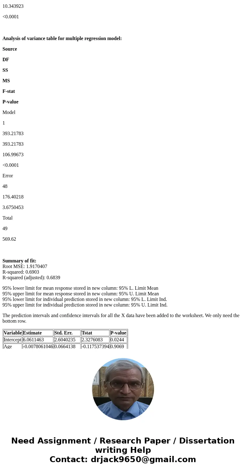
10.343923

<0.0001

Analysis of variance table for multiple regression model:

Source

DF

SS

MS

F-stat

P-value

Model

1

393.21783

393.21783

106.99673

<0.0001

Error

48

176.40218

3.6750453

Total

49

569.62

Summary of fit:
Root MSE: 1.9170407
R-squared: 0.6903
R-squared (adjusted): 0.6839

95% lower limit for mean response stored in new column: 95% L. Limit Mean
95% upper limit for mean response stored in new column: 95% U. Limit Mean
95% lower limit for individual prediction stored in new column: 95% L. Limit Ind.
95% upper limit for individual prediction stored in new column: 95% U. Limit Ind.

The prediction intervals and confidence intervals for all the X data have been added to the worksheet. We only need the bottom row.

Variable	Estimate	Std. Err.	Tstat	P-value
Intercept	6.0611463	2.6040235	2.3276083	0.0244
Age	-0.0078061046	0.0664138	-0.117537394	0.9069
Years	0.60348195	0.09656014	6.2498035	<0.0001
Pay	-0.07024563	0.052370206	-1.3413281	0.1864